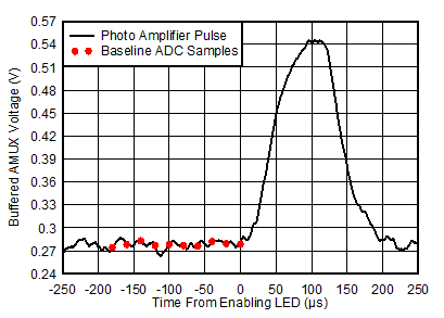
In MATLAB, each waveform is convolved with a symmetric 21-point (210 ns) Hann window to reduce quantization noise caused by the 8-bit oscilloscope ADC. Samples are selected from the waveform using four parameters: first top sample time t_TOP, sampling time interval t_SAMP, number of top samples N_TOP, and number of base samples N_BASE. The base samples are selected starting at time zero, when the LED is enabled, and moving backward in time by t_SAMP increments. The number of base samples used in each SNR calculation is shown in Equation 21. This number sufficiently causes the DC voltage measurement noise to not dominate the total measurement noise.

Figure 4-6 Photo Amplifier Signal With Base ADC Samples Highlighted

Each top sample is subtracted by the average of the base samples. This removes the DC level on the signal. The DC removed signal and ADC samples is shown in Figure 4-7. Two sets of ADC samples are shown: a set centered on the time when the LED is disabled, and an optimal set for maximizing SNR.

Figure 4-7 DC Removed Photo Amplifier Signal With Top ADC Samples Highlighted

Each sample is then scaled by a weight corresponding to the filter used. The averaging filter has equal weights, the matched filter has weights proportional to the noiseless DC-removed pulse shape, and the unconstrained filter can have any weight.

Figure 4-8 Centered and Optimized Digital Filter Weights and ADC Timing

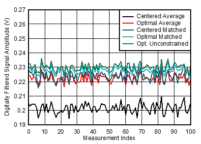
The weighted samples are added together to obtain the signal amplitude. The signal amplitude is obtained for each of the 100 waveforms measured by the oscilloscope.

Figure 4-9 Signal Amplitude After Applying Centered and Optimized Digital Filters

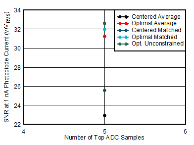
The mean value of the signal amplitude across each waveform is the signal level, and the standard deviation of the signal amplitude across each waveform is the noise level. Dividing the signal level by the noise level calculates the signal-to-noise ratio. The SNR is then divided by the 2.7 nA photodiode current to obtain the SNR at 1 nA photodiode current. The SNR at 1 nA allows anyone to calculate the SNR of the photodiode signal in a system if the system’s photodiode current is known. The SNR at 1 nA is reported here as a unitless ratio and can be converted to decibels by taking the base-10 logarithm and multiplying by 20.

Figure 4-10 SNR at 1 nA Calculated From the Mean and Standard Deviation of Signal Amplitudes

The process is repeated varying different parameters in the system. For example, the data in Figure 4-10 is a portion of the data in Figure 4-13. The rest of the data in Figure 4-13 is collected by varying the number of ADC samples used.

This method of calculating signal-to-noise ratio is formulated into a function and passed to a nonlinear programming solver fminsearch to optimize t_TOP and the unconstrained filter weights. The solver requires an initial guess for the optimized parameters. The first sample time is initialized such that the signal samples are centered on the time when the LED is disabled. The unconstrained filter weights are initialized to the matched filter weights. A first pass optimization is performed by varying the first sample time by t_LED/2 in 1 μs steps and recording the first sample time that achieves the best SNR. This first sample time is then used as the initial guess in the solver. The solver always finds a solution equal to or better than the initial guess, but may not find the optimal configuration.