SPRUIK4A September 2018 – June 2019 TMS320F280021 , TMS320F280021-Q1 , TMS320F280023 , TMS320F280023-Q1 , TMS320F280023C , TMS320F280025 , TMS320F280025-Q1 , TMS320F280025C , TMS320F280025C-Q1 , TMS320F280040-Q1 , TMS320F280040C-Q1 , TMS320F280041 , TMS320F280041-Q1 , TMS320F280041C , TMS320F280041C-Q1 , TMS320F280045 , TMS320F280048-Q1 , TMS320F280048C-Q1 , TMS320F280049 , TMS320F280049-Q1 , TMS320F280049C , TMS320F280049C-Q1 , TMS320F28075 , TMS320F28075-Q1 , TMS320F28076 , TMS320F28374D , TMS320F28374S , TMS320F28375D , TMS320F28375S , TMS320F28375S-Q1 , TMS320F28376D , TMS320F28376S , TMS320F28377D , TMS320F28377D-Q1 , TMS320F28377S , TMS320F28377S-Q1 , TMS320F28378D , TMS320F28378S , TMS320F28379D , TMS320F28379D-Q1 , TMS320F28379S
-
C2000 Software Frequency Response Analyzer (SFRA) Library and Compensation Designer in SDK Framework
- Trademarks
- 1 Introduction
- 2 Installing the SFRA Library
- 3 Module Summary
- 4 Compensation Designer
- 5 Case Study
- 6 Running Software Test Bench Example for SFRA
- 7 Using SFRA Without SFRA GUI Integration
- 8 FAQ
- Revision History
7 Using SFRA Without SFRA GUI Integration
Do these steps to integrate the SFRA in the project:
- Because of resource limitations, some of the applications may not have an SCI port free that is needed by the SFRA GUI.
- In that case, omit the steps for the SFRA GUI integration in Section 3.4.4.
- Integrate the Inject, Collect and background functions as described in Section 3.4.3.
- To start an SFRA sweep, put the SFRA object in the watch window.
- Write SFRA_OBJ.start to 1, when you want the SFRA sweep to start. (This is the alternative to clicking start sweep on the SFRA GUI.)
- Monitor the SFRA_OBJ.FreqIndex variable; it will gradually increment as SFRA sweep is performed.
- Once the SFRA_OBJ.FreqIndex reaches Vec_Length, the SFRA sweep is complete.
- As part of the SFRA initialization, as pointed out in Section 3.4.3, the Open Loop and Plant Magnitude and phase are stored in arrays called.
- Put these in the watch window to inspect and study the response.
- Once the sweep is complete, click on View-> MemoryBrowser inside CCS.
- Inside Memory Browser, enter &freqVect to see the frequency vector and select 32-bit floating point,
- Click on save memory, shown encircled in Figure 23.
- A popup will appear. Select TI data and specify the file name *.dat in the location you prefer.
- Click on Next and specify the address from the memory browser for the start of the array and then the length.
- Make sure 32-bit floating point is selected. Click Finish.
- This will save the data in *.dat file.
- Repeat this step for plantMagVect, plantPhaseVect, olMagVect, olPhaseVect, so you will have 5 *.dat files.
- If you want to use this data in MATLAB or other tools, the data can be populated to an excel file.
- Open the FRAData.xlsx file located at <install directory>\sfra\scripts in excel.
- You can choose to re-name and save the file.
- This excel sheet has four columns, in the first column is the frequency data.
- Open the *dat file that was saved.
- Select the data from the second line onwards to the end of the file and do Ctrl+C to copy the data.
- Open the Excel File, go to the first element under the corresponding vector and do Ctrl+V to copy the array.
- Repeat the steps for each column.
- Once the excel file is updated for all five columns, use the matlab script to import the FRA data. Then, use it inside sisotool to design compensator and carry out stability analysis.
- The file an also be downloaded as a *.csv file and used with the compensation designer tool.
//------- SFRA Related Variables --------
float plantMagVect[SFRA_FREQ_LENGTH];
float plantPhaseVect[SFRA_FREQ_LENGTH];
float olMagVect[SFRA_FREQ_LENGTH];
float olPhaseVect[SFRA_FREQ_LENGTH];
float freqVect[SFRA_FREQ_LENGTH];
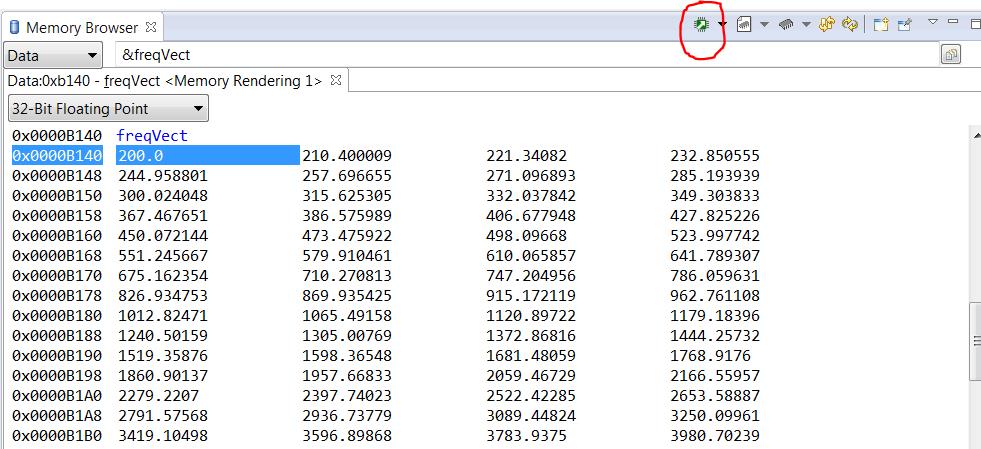 Figure 23. Memory Browser View of Stored SFRA Vectors
 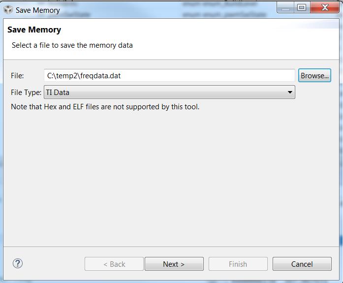 Figure 24. Save Memory Pop-Up Window
 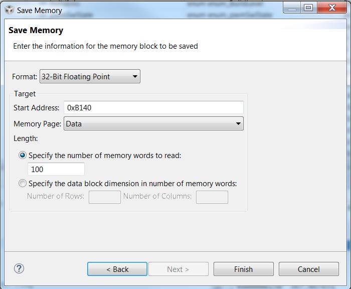 Figure 25. Save Memory Options
 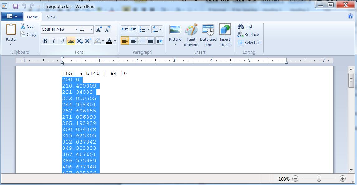 Figure 26. Selecting Data From .dat File to Put in the Excel
 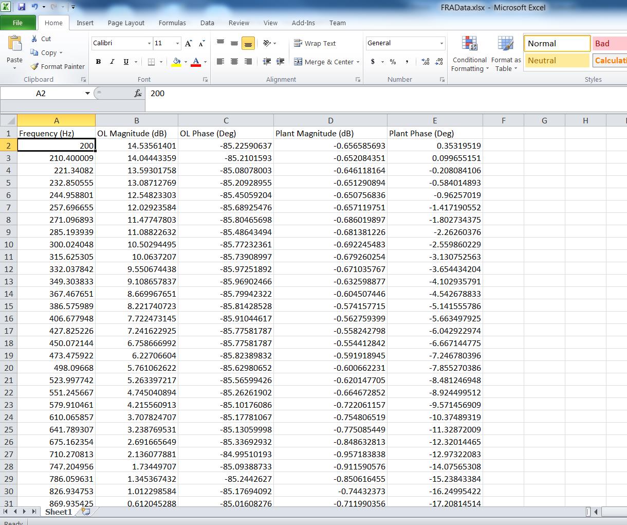 Figure 27. SFRA Data Copied in Excel File